


On conflicting polling results
On conflicting polling results
A causal Bayesian explanation and method for handling conflicts

This is an extensively updated version of an article previously published on my personal blog.
Conflicting polls observed
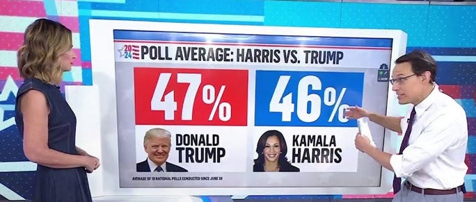
An article by Daniel Jupp last month noted an astonishing difference between what most polls on the US Election were reporting compared to that of a Rasmussen poll:
In the latest polling, every single major polling company and organisation has Queen Kamala and Trump tied, or even Queen K slightly ahead.
Except for one.
Rasmussen has Trump at 62% and Kamala at 35%.
So all the others say even, and Rasmussen says Trump has a huge lead. A giant 27% lead. So what we are seeing here is an outlier, right? The majority of polls must be right and Rasmussen has got it wildly wrong.
No.
For a start a 27% difference in polling results on the same question is not an outlier. An outlier would be maybe a 5 or at its greatest 10% difference from the rest. The Rasmussen difference is too massive to be dismissed as a mere anomaly.
First of all we can be much more explicit in answering the question that Daniel poses when we model the problem using a causal Bayesian network. The solution applies to the completely general problem in which we assume there are just two candidates X (who you could think of as Trump for example) and Y (who you could think of as Harris).
For simplicity, we will assume that there two polls (polls 1 and 2) in which the candidates are more or less tied, and one ‘conflicting’ poll (which you can think of as the Rasmussen poll). Specifically:
In poll 1 both X and Y are tied (i.e. both are at 50%), and in poll 2 Y slightly ahead (so X is 49% and Y is 51%)
In the conflicting poll X is at 62%.
(Binomial) assumptions for inferring the true percentage of X voters from poll results
First we will assume that all the polls are unbiased.
Let p be the ‘true population percentage who favour X’. Unless we really did accurately sample every member of the voting population, we can never know p for certain. But if we assume a poll is unbiased then it is standard to assume that the number of people in the sample supporting X is a Binomial(n, p) distribution where n is the number in the sample. This enables us to predict, for any number between 0 and n, the probability that exactly that number of people in the poll would support X. For example, if p=50 then Figure 1 shows the results for when n=100 and when n=1000
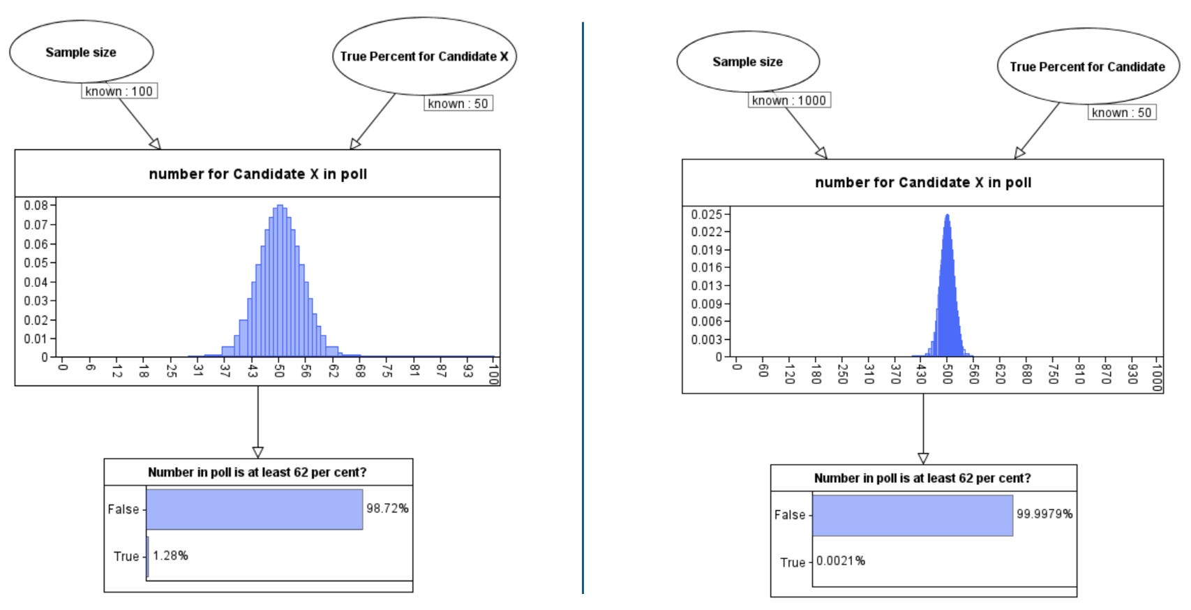
As you can see, the greater the sample size, the higher the probability that the number observed will be close to 50% of the poll size. In the sample size 100, although the probability of observing exactly 50 X voters is only about 0.08 this is still the value with the highest probability.
We can also use this to compute the probability that the number polled will be at least some specific percentage. For example, when the sample size is 100 the probability that at least 62% would support X in the poll is 1.28% (so, that is better than a 1 in 100 chance). However, when the sample size is 1000 the probability that at least 62% would support X in the poll is just 0.0021% (that’s about a 1 in 48,000 chance).
The ‘model’ above is a simple example of a causal Bayesian network and the calculations are examples of ‘forward reasoning’, where we assume we know the true percentage p and use the Binomial theorem to estimate the number of X voters in the poll. But, of course, we do not know p. The true power of Bayesian reasoning is that it allows for ‘backwards reasoning’ where we can ‘learn’ the true value of p from the number of X voters in the poll. In this case, the result is a probability distribution for p.
We have to make some assumptions about the ‘prior’ probability distribution for p. In examples such as this it is reasonable to assume a so-called ‘uniform’ prior which means we assume that p could be any value between 0 and 100% with any value just as likely as any other. With this assumption we get the posterior distributions for p as shown in Figure 2 in the case where we observe 50 supporters of X in a poll of size 100 and then 500 supporters of X in a poll of size 1000.
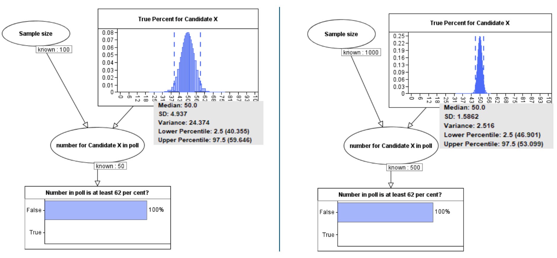
Note that, using a Bayesian inference tool like the one here, we can see the posterior distribution summary statistics. While in both cases the median value is 50, the 95% confidence interval is (40.4 to 59.6) in the case of the smaller poll, and (46.9 to 53.1) in the case of the larger poll. So, for the poll size 1000 this means we can conclude that there is a 95% probability that the true value for p lies between 46.9 and 53.1. It is worth noting that the classical statistical approach to sampling inference and confidence intervals does not allow you to make definitive statements about the probability of the unknown p like this and most people misunderstand confidence intervals in the classical approach. This is explained in this video and it is another reason why we feel the Bayesian approach is superior.
Learning from two polls
We can extend the above causal model to incorporate multiple polls and also the possibility of bias in the polls. The details of the bias factor are explained in the video below, but it’s enough to know that it lies between 0 and 1 with increasingly high values above 0.5 representing increasing poll bias toward people likely to vote X and increasingly low values below 0.5 representing increasing poll bias toward people likely to vote Y. When the bias factor is 0.5 there is no bias.
We will assume that all polls have a sample size of 1000 and (for the time being) that all the polls are unbiased.
So, if we first observe poll 1 showing X at 50% and poll 2 showing X at 49%, then (as shown in Figure 3) we learn that the true percentage for X is a distribution with mean 49.5% and 95% conifence interval 47.3% to 51.7%. In other words, we would conclude that there is a 95% probability that the true percentage for X is between 47.4% and 51.7%.
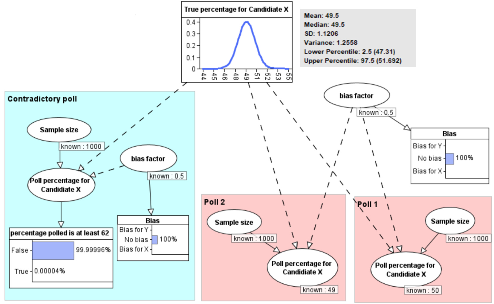
But note that the model also gives us the explict answer to the question Daniel posed: the probability that a different poll would result in at least 62% for X is 0.00004%. That is a 1 in 2.5 million chance. So, as Daniel correctly implied in his conclusion, that is not a feasible outlier. It means there would surely have to be a causal explanation for such a result.
Allowing for (and learning about) possible bias
Daniel suggests that the contradictory poll (Rasmussen) may have posed a different question than the others. While that is something that could be checked, he also raises the possibility of systemic bias as another explanation. If the Rasmusson poll, for example, oversamples Republicans (i.e. those more likely to vote for X) then obviously it will record higher percentages for X than the other polls. Similarly, if there is systemic oversampling of Democrats (i.e. those more likely to vote for Y) in the other polls then obviously they will record lower percentages for X.
Indeed, a couple of weeks after Daniel wrote his article, it does appear that there was evidence that the polls showing there was little to separate Harris and Trump were likely to have been the result of oversampling Democrat supporters.
Because the model explicitly incorporates the possibility of such biases we can revise our conclusions by removing our assumption of no bias. So, if we know nothing about the biases in the polls, then oberving 62% for the contradictory poll results in the revised probabilities shown in Figure 4.
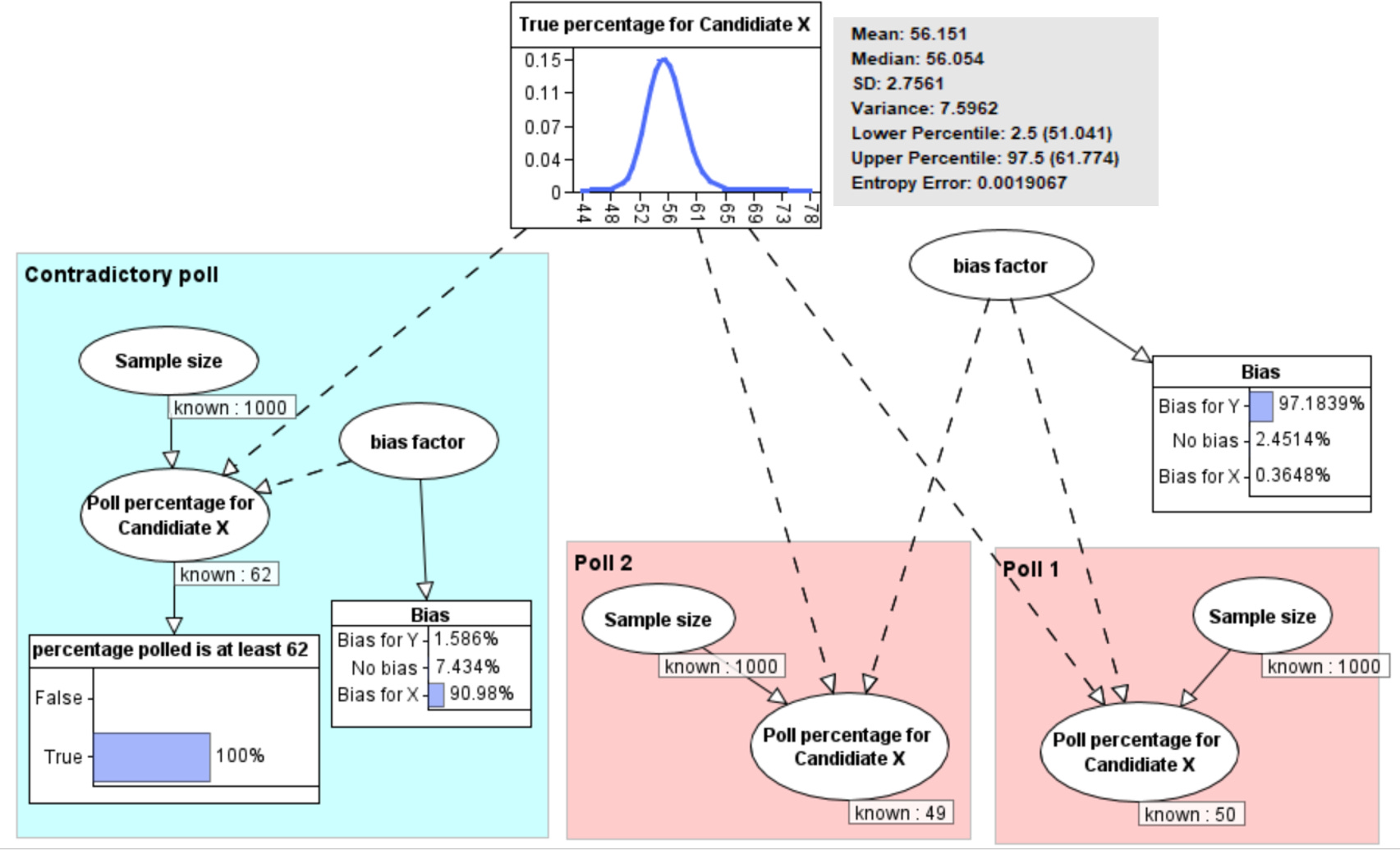
Note that the Bayesian inference enables us to conclude that both sets of polls are biased. There is 91% probability that the contradictory poll is biased in favour of X and a 97% probability that polls 1 and 2 are biased in favour of Y. The reason why there is higher probability that polls 1 and 2 are biased than the contradictory poll is because we are assuming that these polls suffer from the same common bias. The overall impact on the revised probability of the true percentage is that it has mean 56.2% with 95% confidence interval 51% to 61.8%. So even though we now have results from 3 rather than 2 samples, the confidence interval is much wider because of the conflicting results.
But what if we know that the conflicting poll is unbiased and know nothing about any bias in the polls 1 and 2? Then, as shown Figure 5, we learn that there is as 99.98% probability that the other polls are biased in favour of Y and the revised probability of the true percentage is that it has mean 60.5% with 95% confidence interval 57.5% to 63.5%.
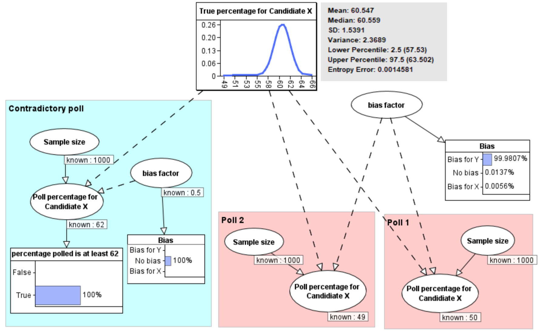
As Daniel notes, there is indeed evidence that, unlike the Rasmussen poll, the other polls have systematically oversampled Democrats.
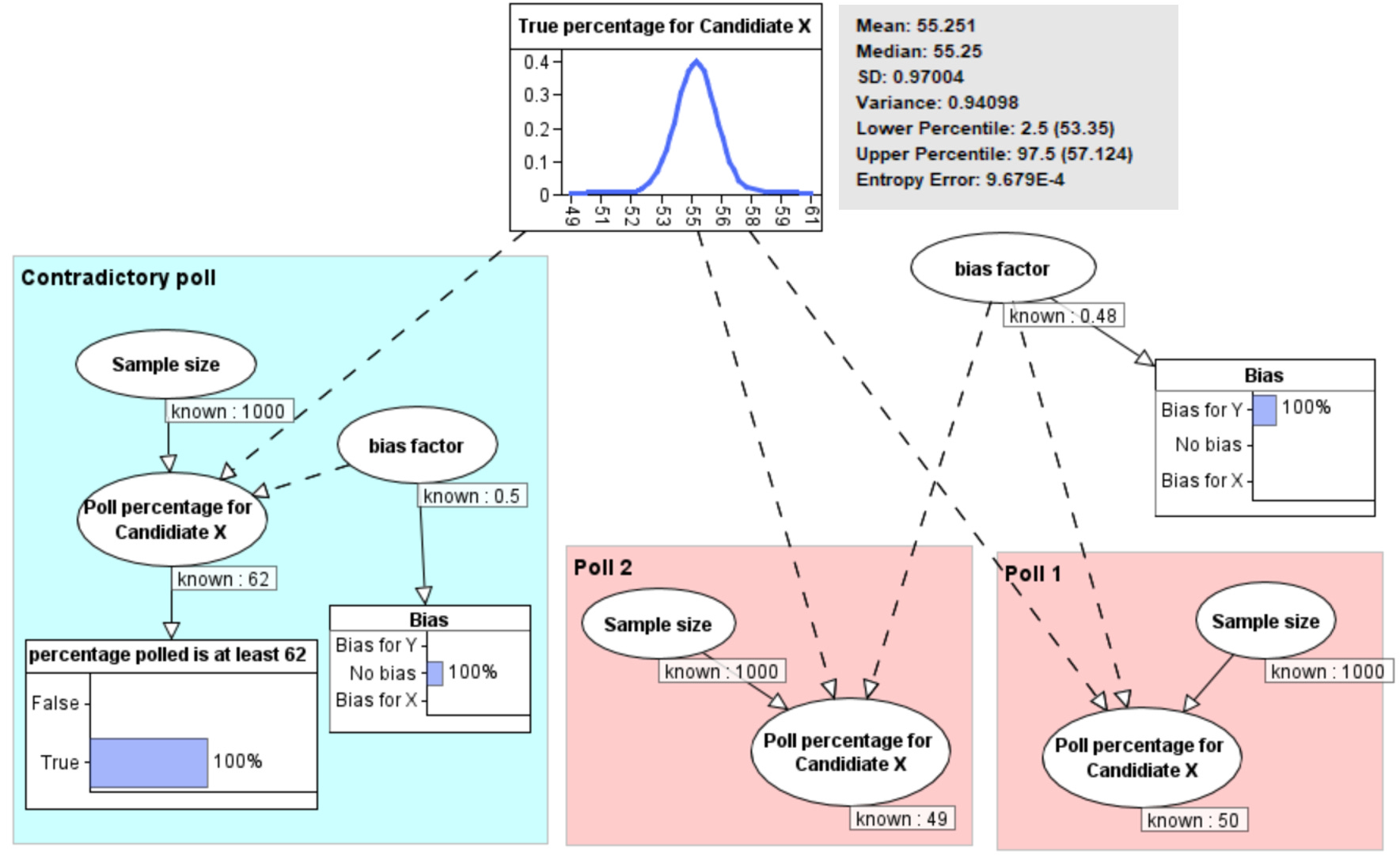
This model can also be used to take account of any known biases. For example, if it was known that the polls 1 and 2 systematically oversampled Democrats, but only by a small amount, say 2%, then we get the results shown in Figure 6. Note that it is now certain there is bias, but the revised probability distribution is no longer so dominated by the (unbiased) contradictory poll result. The revised probability of the true percentage is that it has mean 55.2% with 95% confidence interval 53.3% to 57.1%.
Here is a video demonstration of the above Bayesian network argument (software by agena.ai):
This article by John Ward is also interesting and relevant
I’d never heard of Rasmussen until Steve Kirsch used them for his various Covid polls. Maybe they’re the only pollsters not using leading questions. In terms of predicting the result in November, these traditional nationwide polls are a waste of time. The electoral college means all the action is in the battleground States. The John Ward article is a wild read.